Likelihood Models
Jed Rembold
April 10, 2025
Announcements
- HW5 due on Monday!
- You have everything you need after today!
- Quiz 2 later today
- Poll will be going out about partner preferences on final group
project
- Please respond by end of Monday, as I want to get groups made by Tuesday
- Check-in form this weekend for HW5
Recap
- A Monte Carlo Markov Chain is a semi-random walk wherein the next
step is determined by the current location and a bit of randomness
- Semi-random in the sense that is has a preference to move “uphill”, toward higher parts of the function it is sampling
- By letting the sampling run for a while, and keeping track of where
the walker has been, you can regenerate the walked function by looking
at a histogram of where the walker spent the most time
- Really just regenerate the shape, the scaling will be different
- We can sample the probability of parameters given particular data
(\(P(\theta | D)\)) using Baye’s
theorem
- Requires being able to write out our priors and our likelihood
Today
- How does this all apply to fitting models?
- Writing out our priors and likelihood
- Walking the probability
- Interpretting the results
- MCMC libraries?
Baye Life
Defining the Component Functions
The Prior
The prior dictates the probability of a parameter having a particular value, regardless of the data
If using an unbounded, flat, prior, then it should just return 1 always (0 in ln-space)
If bounded, check the parameters and return 1 (0 in ln-space) if within the bounds or \(-\infty\) otherwise (
-np.infin Python,-Infin R)Pseudo-example:
|||function ln_prior(|||params|||)|||
  if |||illegal condition|||
    return -|||infinity|||
  return 0
|||function ln_prior(|||params|||)||| if |||legal condition||| return 0 return -|||infinity|||
The Likelihood
- The likelihood essentially compares the data our model would output to our actual data
- The goal is to minimize the differences between the two
- Additionally, things are normally scaled by known errors, so that values with more error have less weight
- If our individual data points were arranged around the model with some uncertainty: \[ P(y_i | \theta,\sigma) = \frac{1}{\sqrt{2\pi\sigma^2}} \exp\left(-\frac{(y_i - f(x_i, \theta))^2}{2\sigma^2}\right)\]
- The likelihood is just the sum over all these points. So \[ \log \mathcal{L} = \sum^n_{i=1}\log P(y_i|\theta,\sigma) = \sum^n_{i=1}\left[ -\frac{(y_i - f(x_i,\theta))^2}{2\sigma^2}-\frac{1}{2}\log(2\pi\sigma^2)\right]\]
The Likelihood (In Code)
The ln-likelihood then could look like:
|||function ln_likelihood(|||params, data|||)|||
  m,b = params
  x,y,errY = data # extract data
  y_model = m * x + b # compute model result
  residual = y - y_model # compute the difference
  term1 = - 0.5 * |||log|||(2 * |||pi||| * errY ** 2)
  term2 = - 0.5 * (y - y_model) ** 2 / errY ** 2 )
  return |||sum|||(term1 + term2)
All together now…
Bring both pieces together (since we don’t care about \(P(D)\)):
|||function ln_pdf(|||params, data|||)|||
  p = |||call ln_prior|||
  if p == -|||infinity||| # no sense continuing
    return -|||infinity|||
  return p + ln_likelihood(params, data)
Example Time
Extended Example
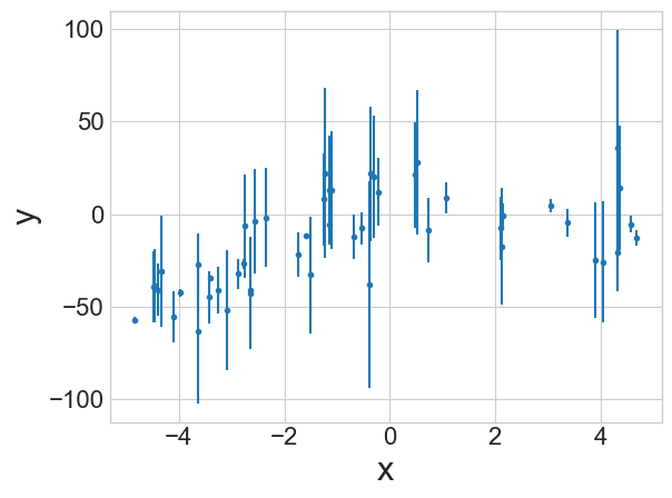
Suppose we want to evaluate the uncertainties in our parameters for a fit to the data to the right.
Our model will look something like: \[y = ax^2 + bx\]
MCMC does not tell you about the quality of a fit. It tells you about the variability in the fit parameters.
Interpreting the Results
Burnin’
- If you have not started your parameter chain near the max, it takes a bit of time for the chain to find its way to the most probably area and start bouncing around
- We don’t care about this initial time period!
- Commonly called burn-in, and we throw away a certain number
of iterations before we start keeping track.
- This generally requires you to look at your parameters vs interations to decide when things reasonably leveled off.
Visualizing the Best Fit with Errors
- There are a few ways you can visualize the best fit model with uncertainties in the parameters reflected
- My go-to looks like:
- Randomly select some number of indices from your leveled chain
- For each index, grab the corresponding parameters and compute your model output with those parameters, appending the result to a list
- Compute the median and standard deviation of the results in your
list, being sure to specify
axis=0 - Plot the median values for your best approximation, and shade the region between the median - std and the median + std
- Alternatively, you could just plot the model output for each of the randomly selected parameter combinations, though I don’t think it looks as nice
MCMC Libraries (Python)
Emcee
- While it isn’t difficult to create our own MCMC sampler, there can
be some benefits to using existing libraries for more complicated use
cases
- Tend to give more intuitive interfaces through which to accomplish the basic tasks that we would want
- In the Python landscape, the main option used is the
emceepackage, which you will probably need to install throughpip Emceeoperates as an abstract data type, wherein you create a sampling object and then can interact with it and run samples using defined methods- In the R landscape, there is the
mcmcpackage, which also seems reasonably strong, though it doesn’t seem to have all of the flexibility ofemcee
Emcee Creation
- When you create the object initially, you need to provide:
- The number of walkers you’d like to generate
- The number of dimensions you’ll be walking (number of parameters)
- The function you’ll be walking (your log posterior)
- Any extra arguments that your function will need beyond the parameters
- A pool should you be using multiprocessing
sampler = emcee.EnsembleSampler(
              num_walkers, num_dims,
              log_function, args=[extra arguments]
              )
Emcee Running
You can then start a sampling run by telling the sampler where all the walkers should begin and how many steps they should take
Generating starting points usually done with some variation of a random gaussian near a starting point:
starts = np.random.multivariate_normal(
            mean = [0,1,10],
            cov = [[1,0,0],[0,0.5,0], [0,0,5]],
            size = num_dims
            )
Then you can just run the sampler:
sampler.run_mcmc(starts, num_iterations)
Emcee Retrieving Chains
You can get the iteration chains back from the sampler after a run using
.get_chain()This will usually return a 3D array, indexing over the parameter, walker, and iteration
Can visualize a particular parameter over all walkers using
plt.plot(sampler.get_chain()[:,:,0], 'k', alpha=0.3)
After examining, will commonly want to discard the burn in and flatten all the individual walkers:
flat_samples = sampler.get_chain(discard=num_dis,
                                 flat=True)