The Classic Periodogram

• Though we’ve touched on it, the classic, or Schuster, periodogram is defined as: \[ P_S(f) = \frac{1}{N}\left|\mathcal{F}(f)\right|^2 \] where \(N\) is the number of discrete measurements in the observing window
• Differs from the power spectrum by a factor of \(\tfrac{1}{N}\), which accounts for the fact that otherwise longer signals will have higher power spectrum values
• Technically, the periodogram is our observational statistic, which serves as an estimator for the underlying power spectrum

Amplitudes and Phases

• Periodograms can help identify the prominent frequencies, but what if you want the other sinusoidal parameters?
  • Amplitude: determined from just the magnitude of the FFT scaled by the number of observations \[ A = \frac{1}{N} \left| \mathcal{F}(f) \right| \times 2 \]
    • The \(\times 2\) comes from the symmetric nature of the FFT
  • Phase: determined from the angle formed by the real and imaginary parts of the FFT \[ \phi = \arctan\left(\frac{\operatorname{Im}(\mathcal{F}(f))}{\operatorname{Re}(\mathcal{F}(f))}\right) \]
    • The returned phase is in radians

The Inverse FFT

• You can also go backwards!
• The Inverse Fourier Transform moves you back from the frequency-domain to the time-domain
• In Python, this is given by ifft
• In R, use the inverse = TRUE flag inside fft
• Make it possible to filter out certain frequencies, and then transform back to a clean signal

Activity!

• I’ve generated noisy data of a single oscillation here.
• Your task is to determine the period/frequency, filter out everything else by setting it to 0, and then transform that signal back and plot it atop the original noise

Common Transforms

Convolutions

• Mathematically, a convolution is defined as: \[ [f * g](t) = \int_{-\infty}^{\infty} f(t)g(t-\tau)\,d\tau \]
• Conceptually, this is the same as:
  • Taking the second function and flipping it about the y-axis
  • Then “sliding” that function across the other, from left to right
  • Each step, summing the area beneath both functions

Visual Convolutions

Why do we care?

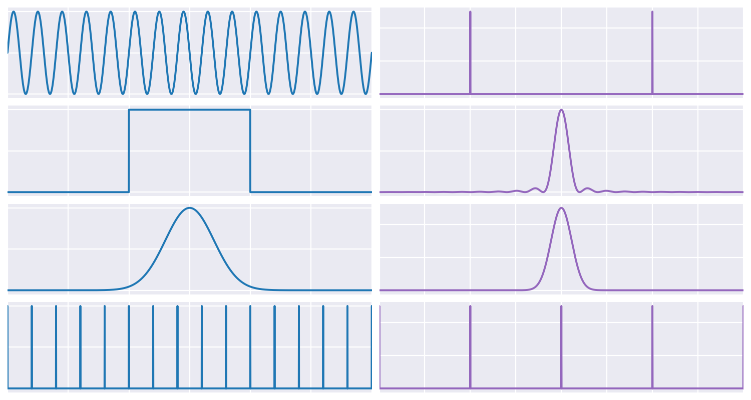
• Fourier Transforms have a particular attribute: \[ \mathcal{F}\{f * g\} = \mathcal{F}\{f\} \cdot \mathcal{F}\{g\} \] or \[ \mathcal{F}\{f \cdot g\} = \mathcal{F}\{f\} * \mathcal{F}\{g\} \]
• In other words: convolutions in one space are the same as just multiplying the function point-wise in the other space

Example 1: Window

Example 2: Discrete Measurements

Our Powers Combined…

• In practice, most real world data consists of both effects:
  • Data was measured over some duration: the window
    • Will cause broadening of our peaks. The narrower the window, the greater the broadening.
  • Data was collected at some frequency: the discrete measurements
    • Will cause aliases of the signal, spaced according to the sampling rate
    • The slower the sampling rate, the more densely packed the aliases

The Nyquist Limit

• Note that if the window of observations gets too small, or the time between observations too large, our Fourier Transform peaks will begin to overlap!
• In this case not all of the frequency information can be recovered
• This is called the Nyquist Limit, and occurs at a frequency of half the sampling frequency
• The FFT algorithm generally measures frequencies up to but not beyond this point, so you shouldn’t see aliases in your results, but your results might not capture what you were hoping to see.

Nyquist Visual

Quiz Time!

• Put your notes away and have just a writing implement and a calculator out!
• Show as much work or your thought process as you can on all problems for the potential of partial credit
• When you are finished you can leave