Maximum Redshift

• Stars are considered “hypervelocity stars” if they have radial speeds of around 500 km/s or higher
• Take a moment to compute how much of a shift this would cause in the \(H_\alpha\) line usually at 656.464 nm.

Gaussians

• Measure peak placement precisely involves fitting a model to the peak
• One of the most common is that of a Gaussian: \[ g(x) = H + A\exp\left(\frac{-(x-x_0)^2}{2\sigma^2}\right) \] where
  • \(H\) is the offset or shift of the baseline
  • \(A\) is the peak height above the baseline (can be negative)
  • \(x_0\) is the \(x\) at which the peak is centered
  • \(\sigma\) is the spread of the peak

The Continuum

• Peaks often show up on areas of the blackbody spectrum that are heavily sloped
• Fitting them well requires “flattening”, or normalizing out this background continuum
• Most common approach is to fit a line or polynomial to just the background (not the peak!) and then divide the entire background by this signal
• If done well, you should get a clean peak sitting on a level surface, ready for fitting
• For velocities or identifying chemical composition, determining \(x_0\) is the most important, as that is the wavelength the peak is centered at

Example Using Solar Spectra

• To illustrate this approach, let’s investigate the \(H_\alpha\) line in the solar spectra given here
• Want to:
  • Establish there is a peak approximately where we expect it
  • Normalize the background
  • Fit a gaussian to determine peak location

Velocity Computing

So what can we observe?

Luminosity

• We measure the apparent brightness \(B\) of an object here at Earth (area under spectra)
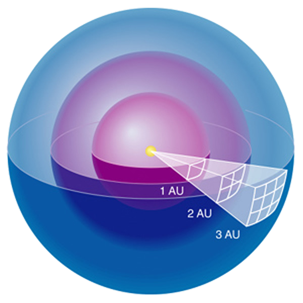
• Like ripples around a dropped rock though, brightness falls off with distance:
  • Unlike pond ripples, the waves spread out radially, so the energy gets spread over a sphere
• Thus the luminosity is: \[ L = 4\pi d^2 \times B \] where \(d\) is the distance
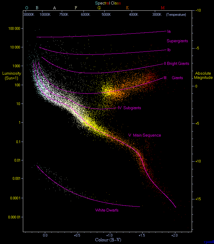
• The range of possible stellar luminosities is huge
  • \(L_{sun} = L_\odot = 4 \times 10^{26}\) W
  • Dimmest at around \(0.000001L_\odot\)
  • Brightest around \(100000L_\odot\)

Stellar Distances

• Initially, coming from parallax
  • Shifts of the foreground relative to the background when the viewpoint changes
• Parallax effects are larger for closer objects, and stars are far away
  • Need as large a baseline as possible: observing during 6 month intervals to be on opposite sides of the Sun
  • Parallax effects from stars are still tiny: generally less than an arcsecond
• A parsec is the distance that corresponds to a parallax angle of 1 arcsecond
  • Equivalent to 3.26 light-years, or 3.26\(\times\) the distance light travels in a year
• Measuring the parallax angle \(p\) in arcseconds gives the distance in parsecs \(d\): \[ d_{pc} = \frac{1}{p_{asec}} \]

Absolute Magnitude

• Astronomers will also use absolute magnitude as a proxy for luminosity
• A star’s absolute magnitude (commonly denoted \(M\)) is the magnitude it would seem to have if it was 10 parsecs away
• Still requires knowing the distance to the star to compute: \[ m - M = 5\log_{10}\left(\frac{d_{pc}}{10}\right) \] where \[ \begin{aligned} M &= \text{ absolute magnitude} \\ m &= \text{ apparent magnitude} \\ d_{pc} &= \text{ distance in pc}\\ \end{aligned} \]

Star Types

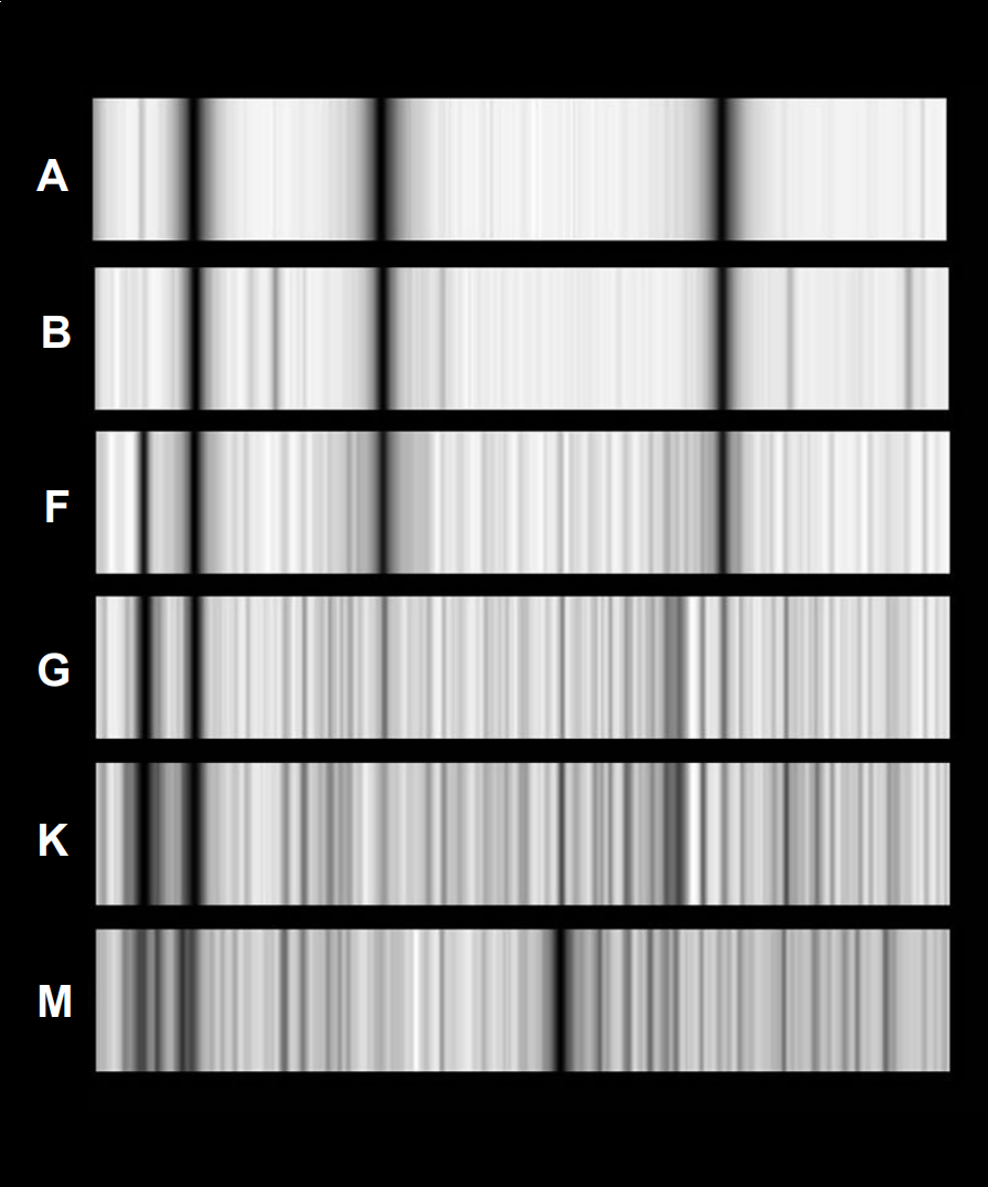
• Stars were originally classified by the strength of their Hydrogen lines
• The strongest were classified type A, all the way down to type O, which showed virtually no hydrogen lines

Scrambling the System

• As more spectra were observed, the H lines were proving to be less reliable in predicting similar properties
• Enter Annie Cannon
  • Hired as one of the Harvard Computers
  • Classified some 350,000 stars (yikes!)
  • Drastically simplied the system and eliminated many classes, focusing mainly on the Balmer line transitions
  • Once the relationship between spectra lines and temperature was understood, the letters were reordered to match the temperature trend

HR Diagrams

HR Diagram

Star Sizes

• Given certain names, you can perhaps guess how stellar size varies in an HR diagram
• But why?
  • Recall that total brightness over some interval of wavelength is measured in watts per square meter
    • This would be the area under a spectra curve
    • This is why brightness drops off as it travels away from the star to us
    • This also means though that the total energy emitted from the surface of the star will depend on the star’s size!
  • The area under the curve depends (heavily) on the temperature \[ L = 4\pi R^2_s \times \sigma T^4 \]

Size Trends

Mass and HR Diagrams